Directory talk:Jon Awbrey/Papers/Differential Logic : Introduction

Quick Overview

Cactus Language for Propositional Logic

The development of differential logic is greatly facilitated by having a conceptually efficient calculus in place at the level of boolean-valued functions and elementary logical propositions. A calculus that is very efficient from both conceptual and computational standpoints is based on just two types of logical connectives, both of variable \(k\!\)-ary scope. The formulas of this calculus map into a species of graph-theoretical structures called painted and rooted cacti (PARCs) that lend visual representation to their functional structure and smooth the path to efficient computation.

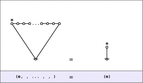
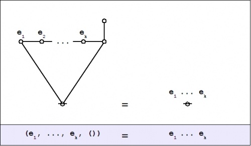
The first kind of propositional expression is a parenthesized sequence of propositional expressions, written as \(\texttt{(} e_1 \texttt{,} e_2 \texttt{,} \ldots \texttt{,} e_{k-1} \texttt{,} e_k \texttt{)}\!\) and read to say that exactly one of the propositions \(e_1, e_2, \ldots, e_{k-1}, e_k\!\) is false, in other words, that their minimal negation is true. A clause of this form maps into a PARC structure called a lobe, in this case, one that is painted with the colors \(e_1, e_2, \ldots, e_{k-1}, e_k\!\) as shown below.

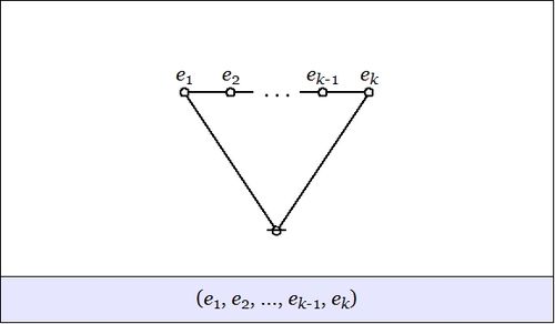
The second kind of propositional expression is a concatenated sequence of propositional expressions, written as \(e_1\ e_2\ \ldots\ e_{k-1}\ e_k\!\) and read to say that all of the propositions \(e_1, e_2, \ldots, e_{k-1}, e_k\!\) are true, in other words, that their logical conjunction is true. A clause of this form maps into a PARC structure called a node, in this case, one that is painted with the colors \(e_1, e_2, \ldots, e_{k-1}, e_k\!\) as shown below.

All other propositional connectives can be obtained through combinations of these two forms. Strictly speaking, the parenthesized form is sufficient to define the concatenated form, making the latter formally dispensable, but it is convenient to maintain it as a concise way of expressing more complicated combinations of parenthesized forms. While working with expressions solely in propositional calculus, it is easiest to use plain parentheses for logical connectives. In contexts where ordinary parentheses are needed for other purposes an alternate typeface \(\texttt{(} \ldots \texttt{)}\!\) may be used for logical operators.

Table 1 collects a sample of basic propositional forms as expressed in terms of cactus language connectives.

\(\text{Table 1.}~~\text{Syntax and Semantics of a Calculus for Propositional Logic}\!\)

\(\text{Graph}\!\)	\(\text{Expression}~\!\)	\(\text{Interpretation}\!\)	\(\text{Other Notations}\!\)
	\(~\!\)	\(\mathrm{true}\!\)	\(1\!\)
	\(\texttt{(~)}\!\)	\(\mathrm{false}\!\)	\(0\!\)
	\(a\!\)	\(a\!\)	\(a\!\)
	\(\texttt{(} a \texttt{)}\!\)	\(\mathrm{not}~ a\!\)	\(\lnot a \quad \bar{a} \quad \tilde{a} \quad a^\prime~\!\)
	\(a ~ b ~ c\!\)	\(a ~\mathrm{and}~ b ~\mathrm{and}~ c\!\)	\(a \land b \land c\!\)
	\(\texttt{((} a \texttt{)(} b \texttt{)(} c \texttt{))}\!\)	\(a ~\mathrm{or}~ b ~\mathrm{or}~ c\!\)	\(a \lor b \lor c\!\)
	\(\texttt{(} a \texttt{(} b \texttt{))}\!\)	\(\begin{matrix} a ~\mathrm{implies}~ b \\[6pt] \mathrm{if}~ a ~\mathrm{then}~ b \end{matrix}\!\)	\(a \Rightarrow b\!\)
	\(\texttt{(} a \texttt{,} b \texttt{)}\!\)	\(\begin{matrix} a ~\mathrm{not~equal~to}~ b \\[6pt] a ~\mathrm{exclusive~or}~ b \end{matrix}\!\)	\(\begin{matrix} a \neq b \\[6pt] a + b \end{matrix}\!\)
	\(\texttt{((} a \texttt{,} b \texttt{))}\!\)	\(\begin{matrix} a ~\mathrm{is~equal~to}~ b \\[6pt] a ~\mathrm{if~and~only~if}~ b \end{matrix}\!\)	\(\begin{matrix} a = b \\[6pt] a \Leftrightarrow b \end{matrix}\!\)
	\(\texttt{(} a \texttt{,} b \texttt{,} c \texttt{)}\!\)	\(\begin{matrix} \mathrm{just~one~of} \\ a, b, c \\ \mathrm{is~false}. \end{matrix}\!\)	\(\begin{matrix} & \bar{a} ~ b ~ c \\ \lor & a ~ \bar{b} ~ c \\ \lor & a ~ b ~ \bar{c} \end{matrix}\!\)
	\(\texttt{((} a \texttt{),(} b \texttt{),(} c \texttt{))}\!\)	\(\begin{matrix} \mathrm{just~one~of} \\ a, b, c \\ \mathrm{is~true}. \\[6pt] \mathrm{partition~all} \\ \mathrm{into}~ a, b, c. \end{matrix}\!\)	\(\begin{matrix} & a ~ \bar{b} ~ \bar{c} \\ \lor & \bar{a} ~ b ~ \bar{c} \\ \lor & \bar{a} ~ \bar{b} ~ c \end{matrix}\!\)
	\(\texttt{(} a \texttt{,(} b \texttt{,} c \texttt{))}\!\)	\(\begin{matrix} \mathrm{oddly~many~of} \\ a, b, c \\ \mathrm{are~true}. \end{matrix}\!\)	\(a + b + c\!\) \(\begin{matrix} & a ~ b ~ c \\ \lor & a ~ \bar{b} ~ \bar{c} \\ \lor & \bar{a} ~ b ~ \bar{c} \\ \lor & \bar{a} ~ \bar{b} ~ c \end{matrix}\!\)
	\(\texttt{(} x \texttt{,(} a \texttt{),(} b \texttt{),(} c \texttt{))}\!\)	\(\begin{matrix} \mathrm{partition}~ x \\ \mathrm{into}~ a, b, c. \\[6pt] \mathrm{genus}~ x ~\mathrm{comprises} \\ \mathrm{species}~ a, b, c. \end{matrix}\!\)	\(\begin{matrix} & \bar{x} ~ \bar{a} ~ \bar{b} ~ \bar{c} \\ \lor & x ~ a ~ \bar{b} ~ \bar{c} \\ \lor & x ~ \bar{a} ~ b ~ \bar{c} \\ \lor & x ~ \bar{a} ~ \bar{b} ~ c \end{matrix}~\!\)

The simplest expression for logical truth is the empty word, usually denoted by \(\boldsymbol\varepsilon\!\) or \(\lambda\!\) in formal languages, where it forms the identity element for concatenation. To make it visible in context, it may be denoted by the equivalent expression \({}^{\backprime\backprime} \texttt{((~))} {}^{\prime\prime},\!\) or, especially if operating in an algebraic context, by a simple \({}^{\backprime\backprime} 1 {}^{\prime\prime}.\!\) Also when working in an algebraic mode, the plus sign \({}^{\backprime\backprime} + {}^{\prime\prime}\!\) may be used for exclusive disjunction. For example, we have the following paraphrases of algebraic expressions by means of parenthesized expressions:

\(\begin{matrix} a + b & = & \texttt{(} a \texttt{,} b \texttt{)} \end{matrix}\!\)

\(\begin{matrix} a + b + c & = & \texttt{(} a \texttt{,(} b \texttt{,} c \texttt{))} & = & \texttt{((} a \texttt{,} b \texttt{),} c \texttt{)} \end{matrix}\!\)

It is important to note that the last expressions are not equivalent to the 3-place parenthesis \(\texttt{(} a \texttt{,} b \texttt{,} c \texttt{)}.\!\)

Differential Expansions of Propositions

Bird's Eye View

An efficient calculus for the realm of logic represented by boolean functions and elementary propositions makes it feasible to compute the finite differences and the differentials of those functions and propositions.

For example, consider a proposition of the form \({}^{\backprime\backprime} \, p ~\mathrm{and}~ q \, {}^{\prime\prime}\!\) that is graphed as two letters attached to a root node:

Written as a string, this is just the concatenation \(p~q\!\).

The proposition \(pq\!\) may be taken as a boolean function \(f(p, q)\!\) having the abstract type \(f : \mathbb{B} \times \mathbb{B} \to \mathbb{B},\!\) where \(\mathbb{B} = \{ 0, 1 \}~\!\) is read in such a way that \(0\!\) means \(\mathrm{false}\!\) and \(1\!\) means \(\mathrm{true}.\!\)

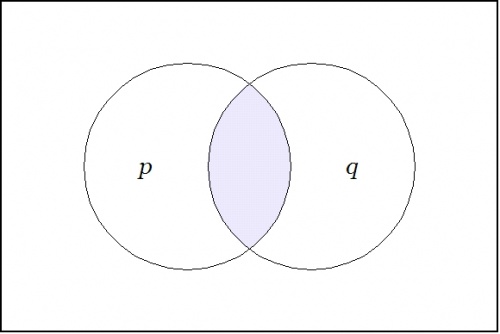
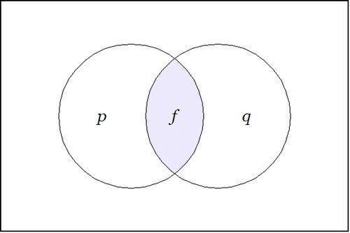
Imagine yourself standing in a fixed cell of the corresponding venn diagram, say, the cell where the proposition \(pq\!\) is true, as shown in the following Figure:

Now ask yourself: What is the value of the proposition \(pq\!\) at a distance of \(\mathrm{d}p\!\) and \(\mathrm{d}q\!\) from the cell \(pq\!\) where you are standing?

Don't think about it — just compute:

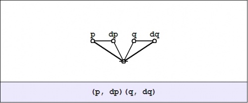
The cactus formula \(\texttt{(p, dp)(q, dq)}\!\) and its corresponding graph arise by substituting \(p + \mathrm{d}p\!\) for \(p\!\) and \(q + \mathrm{d}q\!\) for \(q\!\) in the boolean product or logical conjunction \(pq\!\) and writing the result in the two dialects of cactus syntax. This follows from the fact that the boolean sum \(p + \mathrm{d}p\!\) is equivalent to the logical operation of exclusive disjunction, which parses to a cactus graph of the following form:

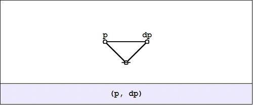
Next question: What is the difference between the value of the proposition \(pq\!\) over there, at a distance of \(\mathrm{d}p\!\) and \(\mathrm{d}q,\!\) and the value of the proposition \(pq\!\) where you are standing, all expressed in the form of a general formula, of course? Here is the appropriate formulation:

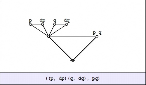
There is one thing that I ought to mention at this point: Computed over \(\mathbb{B},\!\) plus and minus are identical operations. This will make the relation between the differential and the integral parts of the appropriate calculus slightly stranger than usual, but we will get into that later.

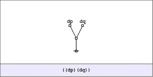
Last question, for now: What is the value of this expression from your current standpoint, that is, evaluated at the point where \(pq\!\) is true? Well, substituting \(1\!\) for \(p\!\) and \(1\!\) for \(q\!\) in the graph amounts to erasing the labels \(p\!\) and \(q\!,\!\) as shown here:

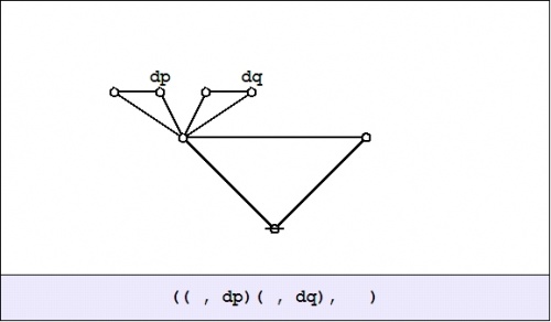
And this is equivalent to the following graph:

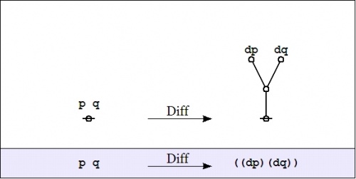
We have just met with the fact that the differential of the and is the or of the differentials.

\(\begin{matrix} p ~\mathrm{and}~ q & \quad & \xrightarrow{\quad\mathrm{Diff}\quad} & \quad & \mathrm{d}p ~\mathrm{or}~ \mathrm{d}q \end{matrix}\!\)

It will be necessary to develop a more refined analysis of that statement directly, but that is roughly the nub of it.

If the form of the above statement reminds you of De Morgan's rule, it is no accident, as differentiation and negation turn out to be closely related operations. Indeed, one can find discussions of logical difference calculus in the Boole–De Morgan correspondence and Peirce also made use of differential operators in a logical context, but the exploration of these ideas has been hampered by a number of factors, not the least of which has been the lack of a syntax that was adequate to handle the complexity of expressions that evolve.

Worm's Eye View

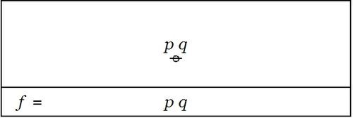
Let's run through the initial example again, this time attempting to interpret the formulas that develop at each stage along the way. We begin with a proposition or a boolean function \(f(p, q) = pq.\!\)

A function like this has an abstract type and a concrete type. The abstract type is what we invoke when we write things like \(f : \mathbb{B} \times \mathbb{B} \to \mathbb{B}\!\) or \(f : \mathbb{B}^2 \to \mathbb{B}.\!\) The concrete type takes into account the qualitative dimensions or the “units” of the case, which can be explained as follows.

Let \(P\!\) be the set of values \(\{ \texttt{(} p \texttt{)},~ p \} ~=~ \{ \mathrm{not}~ p,~ p \} ~\cong~ \mathbb{B}.\!\)

Let \(Q\!\) be the set of values \(\{ \texttt{(} q \texttt{)},~ q \} ~=~ \{ \mathrm{not}~ q,~ q \} ~\cong~ \mathbb{B}.\!\)

Then interpret the usual propositions about \(p, q\!\) as functions of the concrete type \(f : P \times Q \to \mathbb{B}.\!\)

We are going to consider various operators on these functions. Here, an operator \(\mathrm{F}\!\) is a function that takes one function \(f\!\) into another function \(\mathrm{F}f.\!\)

The first couple of operators that we need to consider are logical analogues of the pair that play a founding role in the classical finite difference calculus, namely:

The difference operator \(\Delta,\!\) written here as \(\mathrm{D}.\!\)

The enlargement operator \(\Epsilon,\!\) written here as \(\mathrm{E}.\!\)

These days, \(\mathrm{E}\!\) is more often called the shift operator.

In order to describe the universe in which these operators operate, it is necessary to enlarge the original universe of discourse. Starting from the initial space \(X = P \times Q,\!\) its (first order) differential extension \(\mathrm{E}X\!\) is constructed according to the following specifications:

\(\begin{array}{rcc} \mathrm{E}X & = & X \times \mathrm{d}X \end{array}\!\)

where:

\(\begin{array}{rcc} X & = & P \times Q \\[4pt] \mathrm{d}X & = & \mathrm{d}P \times \mathrm{d}Q \\[4pt] \mathrm{d}P & = & \{ \texttt{(} \mathrm{d}p \texttt{)},~ \mathrm{d}p \} \\[4pt] \mathrm{d}Q & = & \{ \texttt{(} \mathrm{d}q \texttt{)},~ \mathrm{d}q \} \end{array}\!\)

The interpretations of these new symbols can be diverse, but the easiest option for now is just to say that \(\mathrm{d}p\!\) means “change \(p\!\)” and \(\mathrm{d}q\!\) means “change \(q\!\)”.

Drawing a venn diagram for the differential extension \(\mathrm{E}X = X \times \mathrm{d}X\!\) requires four logical dimensions, \(P, Q, \mathrm{d}P, \mathrm{d}Q,\!\) but it is possible to project a suggestion of what the differential features \(\mathrm{d}p\!\) and \(\mathrm{d}q\!\) are about on the 2-dimensional base space \(X = P \times Q\!\) by drawing arrows that cross the boundaries of the basic circles in the venn diagram for \(X,\!\) reading an arrow as \(\mathrm{d}p\!\) if it crosses the boundary between \(p\!\) and \(\texttt{(} p \texttt{)}\!\) in either direction and reading an arrow as \(\mathrm{d}q\!\) if it crosses the boundary between \(q\!\) and \(\texttt{(} q \texttt{)}\!\) in either direction.

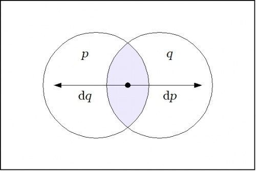
Propositions are formed on differential variables, or any combination of ordinary logical variables and differential logical variables, in the same ways that propositions are formed on ordinary logical variables alone. For example, the proposition \(\texttt{(} \mathrm{d}p \texttt{(} \mathrm{d}q \texttt{))}\!\) says the same thing as \(\mathrm{d}p \Rightarrow \mathrm{d}q,\!\) in other words, that there is no change in \(p\!\) without a change in \(q.\!\)

Given the proposition \(f(p, q)\!\) over the space \(X = P \times Q,\!\) the (first order) enlargement of \(f\!\) is the proposition \(\mathrm{E}f\!\) over the differential extension \(\mathrm{E}X\!\) that is defined by the following formula:

\(\begin{matrix} \mathrm{E}f(p, q, \mathrm{d}p, \mathrm{d}q) & = & f(p + \mathrm{d}p,~ q + \mathrm{d}q) & = & f( \texttt{(} p, \mathrm{d}p \texttt{)},~ \texttt{(} q, \mathrm{d}q \texttt{)} ) \end{matrix}\!\)

In the example \(f(p, q) = pq,\!\) the enlargement \(\mathrm{E}f\!\) is computed as follows:

\(\begin{matrix} \mathrm{E}f(p, q, \mathrm{d}p, \mathrm{d}q) & = & (p + \mathrm{d}p)(q + \mathrm{d}q) & = & \texttt{(} p, \mathrm{d}p \texttt{)(} q, \mathrm{d}q \texttt{)} \end{matrix}\!\)

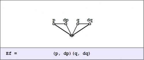
Given the proposition \(f(p, q)\!\) over \(X = P \times Q,\!\) the (first order) difference of \(f\!\) is the proposition \(\mathrm{D}f~\!\) over \(\mathrm{E}X\!\) that is defined by the formula \(\mathrm{D}f = \mathrm{E}f - f,\!\) or, written out in full:

\(\begin{matrix} \mathrm{D}f(p, q, \mathrm{d}p, \mathrm{d}q) & = & f(p + \mathrm{d}p,~ q + \mathrm{d}q) - f(p, q) & = & \texttt{(} f( \texttt{(} p, \mathrm{d}p \texttt{)},~ \texttt{(} q, \mathrm{d}q \texttt{)} ),~ f(p, q) \texttt{)} \end{matrix}\!\)

In the example \(f(p, q) = pq,\!\) the difference \(\mathrm{D}f~\!\) is computed as follows:

\(\begin{matrix} \mathrm{D}f(p, q, \mathrm{d}p, \mathrm{d}q) & = & (p + \mathrm{d}p)(q + \mathrm{d}q) - pq & = & \texttt{((} p, \mathrm{d}p \texttt{)(} q, \mathrm{d}q \texttt{)}, pq \texttt{)} \end{matrix}\!\)

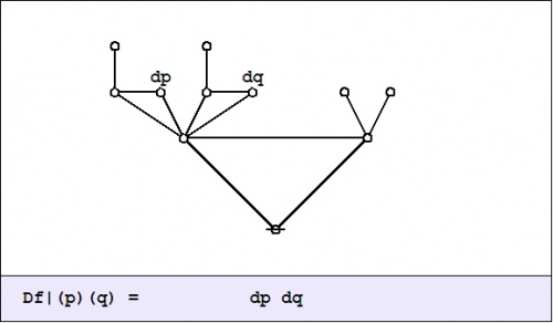
We did not yet go through the trouble to interpret this (first order) difference of conjunction fully, but were happy simply to evaluate it with respect to a single location in the universe of discourse, namely, at the point picked out by the singular proposition \(pq,\!\) that is, at the place where \(p = 1\!\) and \(q = 1.\!\) This evaluation is written in the form \(\mathrm{D}f|_{pq}\!\) or \(\mathrm{D}f|_{(1, 1)},\!\) and we arrived at the locally applicable law that is stated and illustrated as follows:

\(f(p, q) ~=~ pq ~=~ p ~\mathrm{and}~ q \quad \Rightarrow \quad \mathrm{D}f|_{pq} ~=~ \texttt{((} \mathrm{dp} \texttt{)(} \mathrm{d}q \texttt{))} ~=~ \mathrm{d}p ~\mathrm{or}~ \mathrm{d}q\!\)

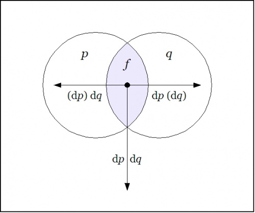
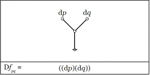
The picture shows the analysis of the inclusive disjunction \(\texttt{((} \mathrm{d}p \texttt{)(} \mathrm{d}q \texttt{))}\!\) into the following exclusive disjunction:

\(\begin{matrix} \mathrm{d}p ~\texttt{(} \mathrm{d}q \texttt{)} & + & \texttt{(} \mathrm{d}p \texttt{)}~ \mathrm{d}q & + & \mathrm{d}p ~\mathrm{d}q \end{matrix}\!\)

The differential proposition that results may be interpreted to say “change \(p\!\) or change \(q\!\) or both”. And this can be recognized as just what you need to do if you happen to find yourself in the center cell and require a complete and detailed description of ways to escape it.

Last time we computed what is variously called the difference map, the difference proposition, or the local proposition \(\mathrm{D}f_x\!\) of the proposition \(f(p, q) = pq\!\) at the point \(x\!\) where \(p = 1\!\) and \(q = 1.\!\)

In the universe \(X = P \times Q,\!\) the four propositions \(pq,~ p \texttt{(} q \texttt{)},~ \texttt{(} p \texttt{)} q,~ \texttt{(} p \texttt{)(} q \texttt{)}\!\) that indicate the “cells”, or the smallest regions of the venn diagram, are called singular propositions. These serve as an alternative notation for naming the points \((1, 1),~ (1, 0),~ (0, 1),~ (0, 0),\!\) respectively.

Thus we can write \(\mathrm{D}f_x = \mathrm{D}f|x = \mathrm{D}f|(1, 1) = \mathrm{D}f|pq,\!\) so long as we know the frame of reference in force.

In the example \(f(p, q) = pq,\!\) the value of the difference proposition \(\mathrm{D}f_x\!\) at each of the four points in \(x \in X\!\) may be computed in graphical fashion as shown below:

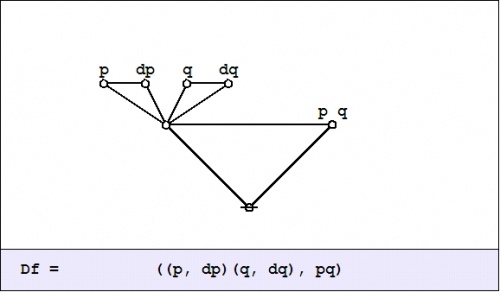
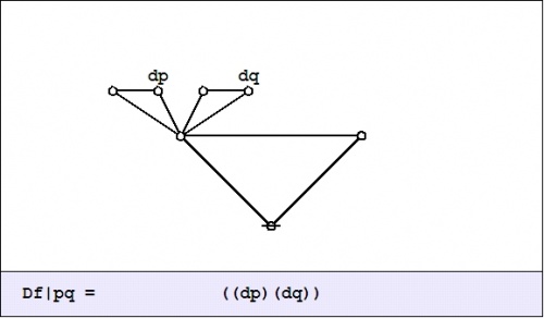
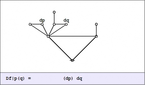
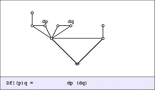
The easy way to visualize the values of these graphical expressions is just to notice the following equivalents:

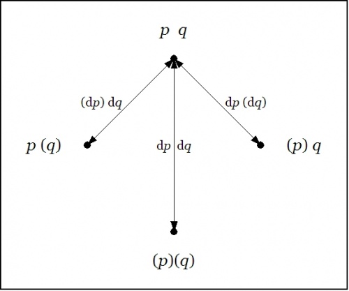
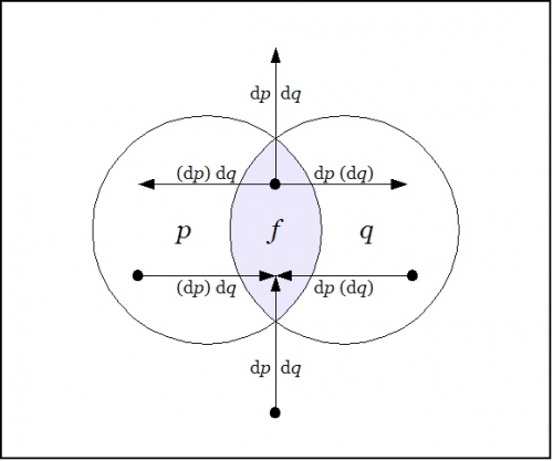
Laying out the arrows on the augmented venn diagram, one gets a picture of a differential vector field.

The Figure shows the points of the extended universe \(\mathrm{E}X = P \times Q \times \mathrm{d}P \times \mathrm{d}Q\!\) that are indicated by the difference map \(\mathrm{D}f : \mathrm{E}X \to \mathbb{B},\!\) namely, the following six points or singular propositions::

\(\begin{array}{rcccc} 1. & p & q & \mathrm{d}p & \mathrm{d}q \\ 2. & p & q & \mathrm{d}p & (\mathrm{d}q) \\ 3. & p & q & (\mathrm{d}p) & \mathrm{d}q \\ 4. & p & (q) & (\mathrm{d}p) & \mathrm{d}q \\ 5. & (p) & q & \mathrm{d}p & (\mathrm{d}q) \\ 6. & (p) & (q) & \mathrm{d}p & \mathrm{d}q \end{array}\!\)

The information borne by \(\mathrm{D}f~\!\) should be clear enough from a survey of these six points — they tell you what you have to do from each point of \(X\!\) in order to change the value borne by \(f(p, q),\!\) that is, the move you have to make in order to reach a point where the value of the proposition \(f(p, q)\!\) is different from what it is where you started.

We have been studying the action of the difference operator \(\mathrm{D}\!\) on propositions of the form \(f : P \times Q \to \mathbb{B},\!\) as illustrated by the example \(f(p, q) = pq\!\) that is known in logic as the conjunction of \(p\!\) and \(q.\!\) The resulting difference map \(\mathrm{D}f~\!\) is a (first order) differential proposition, that is, a proposition of the form \(\mathrm{D}f : P \times Q \times \mathrm{d}P \times \mathrm{d}Q \to \mathbb{B}.\!\)

Abstracting from the augmented venn diagram that shows how the models or satisfying interpretations of \(\mathrm{D}f~\!\) distribute over the extended universe of discourse \(\mathrm{E}X = P \times Q \times \mathrm{d}P \times \mathrm{d}Q,\!\) the difference map \(\mathrm{D}f~\!\) can be represented in the form of a digraph or directed graph, one whose points are labeled with the elements of \(X = P \times Q\!\) and whose arrows are labeled with the elements of \(\mathrm{d}X = \mathrm{d}P \times \mathrm{d}Q,\!\) as shown in the following Figure.

\(\begin{array}{rcccccc} f & = & p & \cdot & q \\[4pt] \mathrm{D}f & = & p & \cdot & q & \cdot & ((\mathrm{d}p)(\mathrm{d}q)) \\[4pt] & + & p & \cdot & (q) & \cdot & ~(\mathrm{d}p)~\mathrm{d}q~~ \\[4pt] & + & (p) & \cdot & q & \cdot & ~~\mathrm{d}p~(\mathrm{d}q)~ \\[4pt] & + & (p) & \cdot & (q) & \cdot & ~~\mathrm{d}p~~\mathrm{d}q~~ \end{array}\!\)

Any proposition worth its salt can be analyzed from many different points of view, any one of which has the potential to reveal an unsuspected aspect of the proposition's meaning. We will encounter more and more of these alternative readings as we go.

The enlargement or shift operator \(\mathrm{E}\!\) exhibits a wealth of interesting and useful properties in its own right, so it pays to examine a few of the more salient features that play out on the surface of our initial example, \(f(p, q) = pq.\!\)

A suitably generic definition of the extended universe of discourse is afforded by the following set-up:

\(\begin{array}{lccl} \text{Let} & X & = & X_1 \times \ldots \times X_k. \\[6pt] \text{Let} & \mathrm{d}X & = & \mathrm{d}X_1 \times \ldots \times \mathrm{d}X_k. \\[6pt] \text{Then} & \mathrm{E}X & = & X \times \mathrm{d}X \\[6pt] & & = & X_1 \times \ldots \times X_k ~\times~ \mathrm{d}X_1 \times \ldots \times \mathrm{d}X_k \end{array}\!\)

For a proposition of the form \(f : X_1 \times \ldots \times X_k \to \mathbb{B},\!\) the (first order) enlargement of \(f\!\) is the proposition \(\mathrm{E}f : \mathrm{E}X \to \mathbb{B}\!\) that is defined by the following equation:

\(\begin{array}{l} \mathrm{E}f(x_1, \ldots, x_k, \mathrm{d}x_1, \ldots, \mathrm{d}x_k) \\[6pt] = \quad f(x_1 + \mathrm{d}x_1, \ldots, x_k + \mathrm{d}x_k) \\[6pt] = \quad f( \texttt{(} x_1, \mathrm{d}x_1 \texttt{)}, \ldots, \texttt{(} x_k, \mathrm{d}x_k \texttt{)} ) \end{array}\!\)

The differential variables \(\mathrm{d}x_j\!\) are boolean variables of the same basic type as the ordinary variables \(x_j.\!\) Although it is conventional to distinguish the (first order) differential variables with the operative prefix “\(\mathrm{d}\!\)” this way of notating differential variables is entirely optional. It is their existence in particular relations to the initial variables, not their names, that defines them as differential variables.

In the example of logical conjunction, \(f(p, q) = pq,\!\) the enlargement \(\mathrm{E}f\!\) is formulated as follows:

\(\begin{array}{l} \mathrm{E}f(p, q, \mathrm{d}p, \mathrm{d}q) \\[6pt] = \quad (p + \mathrm{d}p)(q + \mathrm{d}q) \\[6pt] = \quad \texttt{(} p, \mathrm{d}p \texttt{)(} q, \mathrm{d}q \texttt{)} \end{array}\!\)

Given that this expression uses nothing more than the boolean ring operations of addition and multiplication, it is permissible to “multiply things out” in the usual manner to arrive at the following result:

\(\begin{matrix} \mathrm{E}f(p, q, \mathrm{d}p, \mathrm{d}q) & = & p~q & + & p~\mathrm{d}q & + & q~\mathrm{d}p & + & \mathrm{d}p~\mathrm{d}q \end{matrix}\!\)

To understand what the enlarged or shifted proposition means in logical terms, it serves to go back and analyze the above expression for \(\mathrm{E}f\!\) in the same way that we did for \(\mathrm{D}f.\!\) Toward that end, the value of \(\mathrm{E}f_x\!\) at each \(x \in X\!\) may be computed in graphical fashion as shown below:

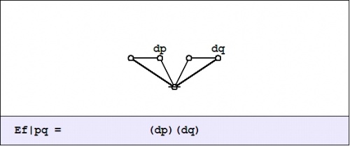
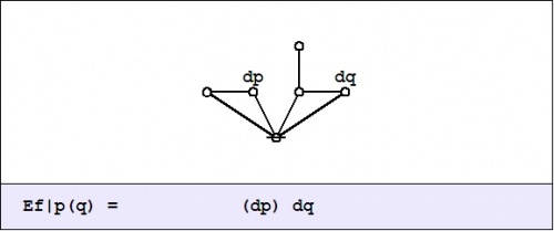
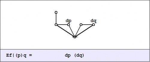
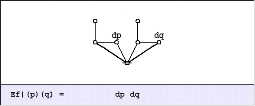
Given the data that develops in this form of analysis, the disjoined ingredients can now be folded back into a boolean expansion or a disjunctive normal form (DNF) that is equivalent to the enlarged proposition \(\mathrm{E}f.\!\)

\(\begin{matrix} \mathrm{E}f & = & pq \cdot \mathrm{E}f_{pq} & + & p(q) \cdot \mathrm{E}f_{p(q)} & + & (p)q \cdot \mathrm{E}f_{(p)q} & + & (p)(q) \cdot \mathrm{E}f_{(p)(q)} \end{matrix}\!\)

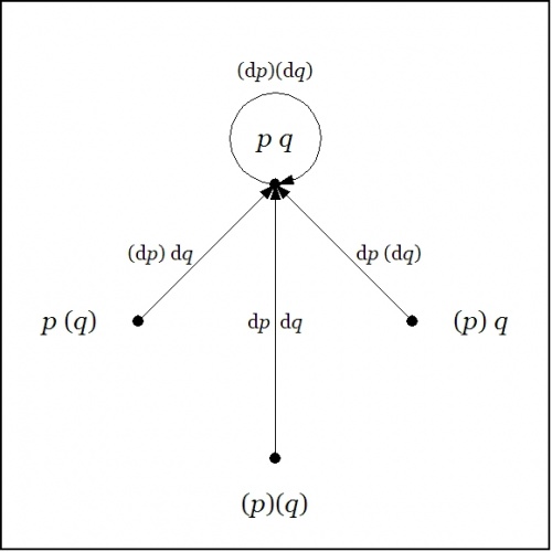
Here is a summary of the result, illustrated by means of a digraph picture, where the “no change” element \((\mathrm{d}p)(\mathrm{d}q)\!\) is drawn as a loop at the point \(p~q.\!\)

\(\begin{array}{rcccccc} f & = & p & \cdot & q \\[4pt] \mathrm{E}f & = & p & \cdot & q & \cdot & (\mathrm{d}p)(\mathrm{d}q) \\[4pt] & + & p & \cdot & (q) & \cdot & (\mathrm{d}p)~\mathrm{d}q~ \\[4pt] & + & (p) & \cdot & q & \cdot & ~\mathrm{d}p~(\mathrm{d}q) \\[4pt] & + & (p) & \cdot & (q) & \cdot & ~\mathrm{d}p~~\mathrm{d}q~\end{array}\!\)

We may understand the enlarged proposition \(\mathrm{E}f\!\) as telling us all the different ways to reach a model of the proposition \(f\!\) from each point of the universe \(X.\!\)

Propositional Forms on Two Variables

To broaden our experience with simple examples, let us examine the sixteen functions of concrete type \(P \times Q \to \mathbb{B}\!\) and abstract type \(\mathbb{B} \times \mathbb{B} \to \mathbb{B}.\!\) A few Tables are set here that detail the actions of \(\mathrm{E}\!\) and \(\mathrm{D}\!\) on each of these functions, allowing us to view the results in several different ways.

Tables A1 and A2 show two ways of arranging the 16 boolean functions on two variables, giving equivalent expressions for each function in several different systems of notation.

\(\text{Table A1.}~~\text{Propositional Forms on Two Variables}\!\)

\(\mathcal{L}_1\!\) \(\text{Decimal}\!\)	\(\mathcal{L}_2\!\) \(\text{Binary}\!\)	\(\mathcal{L}_3\!\) \(\text{Vector}\!\)	\(\mathcal{L}_4\!\) \(\text{Cactus}\!\)	\(\mathcal{L}_5\!\) \(\text{English}\!\)	\(\mathcal{L}_6~\!\) \(\text{Ordinary}\!\)
	\(p\colon\!\)	\(1~1~0~0\!\)
	\(q\colon\!\)	\(1~0~1~0\!\)
\(\begin{matrix} f_0 \\[4pt] f_1 \\[4pt] f_2 \\[4pt] f_3 \\[4pt] f_4 \\[4pt] f_5 \\[4pt] f_6 \\[4pt] f_7 \end{matrix}\!\)	\(\begin{matrix} f_{0000} \\[4pt] f_{0001} \\[4pt] f_{0010} \\[4pt] f_{0011} \\[4pt] f_{0100} \\[4pt] f_{0101} \\[4pt] f_{0110} \\[4pt] f_{0111} \end{matrix}\!\)	\(\begin{matrix} 0~0~0~0 \\[4pt] 0~0~0~1 \\[4pt] 0~0~1~0 \\[4pt] 0~0~1~1 \\[4pt] 0~1~0~0 \\[4pt] 0~1~0~1 \\[4pt] 0~1~1~0 \\[4pt] 0~1~1~1 \end{matrix}\!\)	\(\begin{matrix} (~) \\[4pt] (p)(q) \\[4pt] (p)~q~ \\[4pt] (p)[[User:Jon Awbrey|Jon Awbrey]] ([[User talk:Jon Awbrey|talk]]) \\[4pt] ~p~(q) \\[4pt] [[User:Jon Awbrey|Jon Awbrey]] ([[User talk:Jon Awbrey|talk]])(q) \\[4pt] (p,~q) \\[4pt] (p~~q) \end{matrix}\!\)	\(\begin{matrix} \text{false} \\[4pt] \text{neither}~ p ~\text{nor}~ q \\[4pt] q ~\text{without}~ p \\[4pt] \text{not}~ p \\[4pt] p ~\text{without}~ q \\[4pt] \text{not}~ q \\[4pt] p ~\text{not equal to}~ q \\[4pt] \text{not both}~ p ~\text{and}~ q \end{matrix}\!\)	\(\begin{matrix} 0 \\[4pt] \lnot p \land \lnot q \\[4pt] \lnot p \land q \\[4pt] \lnot p \\[4pt] p \land \lnot q \\[4pt] \lnot q \\[4pt] p \ne q \\[4pt] \lnot p \lor \lnot q \end{matrix}\!\)
\(\begin{matrix} f_8 \\[4pt] f_9 \\[4pt] f_{10} \\[4pt] f_{11} \\[4pt] f_{12} \\[4pt] f_{13} \\[4pt] f_{14} \\[4pt] f_{15} \end{matrix}\!\)	\(\begin{matrix} f_{1000} \\[4pt] f_{1001} \\[4pt] f_{1010} \\[4pt] f_{1011} \\[4pt] f_{1100} \\[4pt] f_{1101} \\[4pt] f_{1110} \\[4pt] f_{1111} \end{matrix}\!\)	\(\begin{matrix} 1~0~0~0 \\[4pt] 1~0~0~1 \\[4pt] 1~0~1~0 \\[4pt] 1~0~1~1 \\[4pt] 1~1~0~0 \\[4pt] 1~1~0~1 \\[4pt] 1~1~1~0 \\[4pt] 1~1~1~1 \end{matrix}\!\)	\(\begin{matrix} ~~p~~q~~ \\[4pt] ((p,~q)) \\[4pt] 18:36, 29 November 2015 (UTC)q~~ \\[4pt] ~(p~(q)) \\[4pt] ~~p18:36, 29 November 2015 (UTC) \\[4pt] ((p)~q)~ \\[4pt] ((p)(q)) \\[4pt] ((~)) \end{matrix}\!\)	\(\begin{matrix} p ~\text{and}~ q \\[4pt] p ~\text{equal to}~ q \\[4pt] q \\[4pt] \text{not}~ p ~\text{without}~ q \\[4pt] p \\[4pt] \text{not}~ q ~\text{without}~ p \\[4pt] p ~\text{or}~ q \\[4pt] \text{true} \end{matrix}\!\)	\(\begin{matrix} p \land q \\[4pt] p = q \\[4pt] q \\[4pt] p \Rightarrow q \\[4pt] p \\[4pt] p \Leftarrow q \\[4pt] p \lor q \\[4pt] 1 \end{matrix}\!\)

\(\text{Table A2.}~~\text{Propositional Forms on Two Variables}\!\)

\(\mathcal{L}_1\!\) \(\text{Decimal}\!\)	\(\mathcal{L}_2\!\) \(\text{Binary}\!\)	\(\mathcal{L}_3\!\) \(\text{Vector}\!\)	\(\mathcal{L}_4\!\) \(\text{Cactus}\!\)	\(\mathcal{L}_5\!\) \(\text{English}\!\)	\(\mathcal{L}_6~\!\) \(\text{Ordinary}\!\)
	\(p\colon\!\)	\(1~1~0~0\!\)
	\(q\colon\!\)	\(1~0~1~0\!\)
\(f_0\!\)	\(f_{0000}\!\)	\(0~0~0~0\!\)	\((~)\!\)	\(\text{false}\!\)	\(0\!\)
\(\begin{matrix} f_1 \\[4pt] f_2 \\[4pt] f_4 \\[4pt] f_8 \end{matrix}\!\)	\(\begin{matrix} f_{0001} \\[4pt] f_{0010} \\[4pt] f_{0100} \\[4pt] f_{1000} \end{matrix}\!\)	\(\begin{matrix} 0~0~0~1 \\[4pt] 0~0~1~0 \\[4pt] 0~1~0~0 \\[4pt] 1~0~0~0 \end{matrix}\!\)	\(\begin{matrix} (p)(q) \\[4pt] (p)~q~ \\[4pt] ~p~(q) \\[4pt] ~p~~q~ \end{matrix}\!\)	\(\begin{matrix} \text{neither}~ p ~\text{nor}~ q \\[4pt] q ~\text{without}~ p \\[4pt] p ~\text{without}~ q \\[4pt] p ~\text{and}~ q \end{matrix}\!\)	\(\begin{matrix} \lnot p \land \lnot q \\[4pt] \lnot p \land q \\[4pt] p \land \lnot q \\[4pt] p \land q \end{matrix}\!\)
\(\begin{matrix} f_3 \\[4pt] f_{12} \end{matrix}\!\)	\(\begin{matrix} f_{0011} \\[4pt] f_{1100} \end{matrix}\!\)	\(\begin{matrix} 0~0~1~1 \\[4pt] 1~1~0~0 \end{matrix}\!\)	\(\begin{matrix} (p) \\[4pt] ~p~ \end{matrix}\!\)	\(\begin{matrix} \text{not}~ p \\[4pt] p \end{matrix}\!\)	\(\begin{matrix} \lnot p \\[4pt] p \end{matrix}\!\)
\(\begin{matrix} f_6 \\[4pt] f_9 \end{matrix}\!\)	\(\begin{matrix} f_{0110} \\[4pt] f_{1001} \end{matrix}\!\)	\(\begin{matrix} 0~1~1~0 \\[4pt] 1~0~0~1 \end{matrix}\!\)	\(\begin{matrix} ~(p,~q)~ \\[4pt] ((p,~q)) \end{matrix}\!\)	\(\begin{matrix} p ~\text{not equal to}~ q \\[4pt] p ~\text{equal to}~ q \end{matrix}\!\)	\(\begin{matrix} p \ne q \\[4pt] p = q \end{matrix}\!\)
\(\begin{matrix} f_5 \\[4pt] f_{10} \end{matrix}\!\)	\(\begin{matrix} f_{0101} \\[4pt] f_{1010} \end{matrix}\!\)	\(\begin{matrix} 0~1~0~1 \\[4pt] 1~0~1~0 \end{matrix}\!\)	\(\begin{matrix} (q) \\[4pt] ~q~ \end{matrix}\!\)	\(\begin{matrix} \text{not}~ q \\[4pt] q \end{matrix}\!\)	\(\begin{matrix} \lnot q \\[4pt] q \end{matrix}\!\)
\(\begin{matrix} f_7 \\[4pt] f_{11} \\[4pt] f_{13} \\[4pt] f_{14} \end{matrix}\!\)	\(\begin{matrix} f_{0111} \\[4pt] f_{1011} \\[4pt] f_{1101} \\[4pt] f_{1110} \end{matrix}\!\)	\(\begin{matrix} 0~1~1~1 \\[4pt] 1~0~1~1 \\[4pt] 1~1~0~1 \\[4pt] 1~1~1~0 \end{matrix}\!\)	\(\begin{matrix} ~(p~~q)~ \\[4pt] ~(p~(q)) \\[4pt] ((p)~q)~ \\[4pt] ((p)(q)) \end{matrix}\!\)	\(\begin{matrix} \text{not both}~ p ~\text{and}~ q \\[4pt] \text{not}~ p ~\text{without}~ q \\[4pt] \text{not}~ q ~\text{without}~ p \\[4pt] p ~\text{or}~ q \end{matrix}\!\)	\(\begin{matrix} \lnot p \lor \lnot q \\[4pt] p \Rightarrow q \\[4pt] p \Leftarrow q \\[4pt] p \lor q \end{matrix}\!\)
\(f_{15}\!\)	\(f_{1111}\!\)	\(1~1~1~1\!\)	\(((~))\!\)	\(\text{true}\!\)	\(1\!\)

Transforms Expanded over Differential Features

The next four Tables expand the expressions of \(\mathrm{E}f\!\) and \(\mathrm{D}f~\!\) in two different ways, for each of the sixteen functions. Notice that the functions are given in a different order, partitioned into seven natural classes by a group action.

\(\text{Table A3.}~~\mathrm{E}f ~\text{Expanded over Differential Features}~ \{ \mathrm{d}p, \mathrm{d}q \}\!\)

	\(f\!\)	\(\mathrm{T}_{11} f\!\) \(\mathrm{E}f|_{\mathrm{d}p~\mathrm{d}q}\!\)	\(\mathrm{T}_{10} f\!\) \(\mathrm{E}f|_{\mathrm{d}p(\mathrm{d}q)}\!\)	\(\mathrm{T}_{01} f\!\) \(\mathrm{E}f|_{(\mathrm{d}p)\mathrm{d}q}\!\)	\(\mathrm{T}_{00} f\!\) \(\mathrm{E}f|_{(\mathrm{d}p)(\mathrm{d}q)}\!\)
\(f_0\!\)	\((~)\!\)	\((~)\!\)	\((~)\!\)	\((~)\!\)	\((~)\!\)
\(\begin{matrix} f_1 \\[4pt] f_2 \\[4pt] f_4 \\[4pt] f_8 \end{matrix}\!\)	\(\begin{matrix} (p)(q) \\[4pt] (p)~q~ \\[4pt] ~p~(q) \\[4pt] ~p~~q~ \end{matrix}\!\)	\(\begin{matrix} ~p~~q~ \\[4pt] ~p~(q) \\[4pt] (p)~q~ \\[4pt] (p)(q) \end{matrix}\!\)	\(\begin{matrix} ~p~(q) \\[4pt] ~p~~q~ \\[4pt] (p)(q) \\[4pt] (p)~q~ \end{matrix}\!\)	\(\begin{matrix} (p)~q~ \\[4pt] (p)(q) \\[4pt] ~p~~q~ \\[4pt] ~p~(q) \end{matrix}\!\)	\(\begin{matrix} (p)(q) \\[4pt] (p)~q~ \\[4pt] ~p~(q) \\[4pt] ~p~~q~ \end{matrix}\!\)
\(\begin{matrix} f_3 \\[4pt] f_{12} \end{matrix}\!\)	\(\begin{matrix} (p) \\[4pt] ~p~ \end{matrix}\!\)	\(\begin{matrix} ~p~ \\[4pt] (p) \end{matrix}\!\)	\(\begin{matrix} ~p~ \\[4pt] (p) \end{matrix}\!\)	\(\begin{matrix} (p) \\[4pt] ~p~ \end{matrix}\!\)	\(\begin{matrix} (p) \\[4pt] ~p~ \end{matrix}\!\)
\(\begin{matrix} f_6 \\[4pt] f_9 \end{matrix}\!\)	\(\begin{matrix} ~(p,~q)~ \\[4pt] ((p,~q)) \end{matrix}\!\)	\(\begin{matrix} ~(p,~q)~ \\[4pt] ((p,~q)) \end{matrix}\!\)	\(\begin{matrix} ((p,~q)) \\[4pt] ~(p,~q)~ \end{matrix}\!\)	\(\begin{matrix} ((p,~q)) \\[4pt] ~(p,~q)~ \end{matrix}\!\)	\(\begin{matrix} ~(p,~q)~ \\[4pt] ((p,~q)) \end{matrix}\!\)
\(\begin{matrix} f_5 \\[4pt] f_{10} \end{matrix}\!\)	\(\begin{matrix} (q) \\[4pt] ~q~ \end{matrix}\!\)	\(\begin{matrix} ~q~ \\[4pt] (q) \end{matrix}\!\)	\(\begin{matrix} (q) \\[4pt] ~q~ \end{matrix}\!\)	\(\begin{matrix} ~q~ \\[4pt] (q) \end{matrix}\!\)	\(\begin{matrix} (q) \\[4pt] ~q~ \end{matrix}\!\)
\(\begin{matrix} f_7 \\[4pt] f_{11} \\[4pt] f_{13} \\[4pt] f_{14} \end{matrix}\!\)	\(\begin{matrix} (~p~~q~) \\[4pt] (~p~(q)) \\[4pt] ((p)~q~) \\[4pt] ((p)(q)) \end{matrix}\!\)	\(\begin{matrix} ((p)(q)) \\[4pt] ((p)~q~) \\[4pt] (~p~(q)) \\[4pt] (~p~~q~) \end{matrix}\!\)	\(\begin{matrix} ((p)~q~) \\[4pt] ((p)(q)) \\[4pt] (~p~~q~) \\[4pt] (~p~(q)) \end{matrix}\!\)	\(\begin{matrix} (~p~(q)) \\[4pt] (~p~~q~) \\[4pt] ((p)(q)) \\[4pt] ((p)~q~) \end{matrix}\!\)	\(\begin{matrix} (~p~~q~) \\[4pt] (~p~(q)) \\[4pt] ((p)~q~) \\[4pt] ((p)(q)) \end{matrix}\!\)
\(f_{15}\!\)	\(((~))\!\)	\(((~))\!\)	\(((~))\!\)	\(((~))\!\)	\(((~))\!\)
\(\text{Fixed Point Total}\!\)		\(4\!\)	\(4\!\)	\(4\!\)	\(16\!\)

\(\text{Table A4.}~~\mathrm{D}f ~\text{Expanded over Differential Features}~ \{ \mathrm{d}p, \mathrm{d}q \}\!\)

	\(f\!\)	\(\mathrm{D}f|_{\mathrm{d}p~\mathrm{d}q}\!\)	\(\mathrm{D}f|_{\mathrm{d}p(\mathrm{d}q)}\!\)	\(\mathrm{D}f|_{(\mathrm{d}p)\mathrm{d}q}\!\)	\(\mathrm{D}f|_{(\mathrm{d}p)(\mathrm{d}q)}\!\)
\(f_0\!\)	\((~)\!\)	\((~)\!\)	\((~)\!\)	\((~)\!\)	\((~)\!\)
\(\begin{matrix} f_1 \\[4pt] f_2 \\[4pt] f_4 \\[4pt] f_8 \end{matrix}\!\)	\(\begin{matrix} (p)(q) \\[4pt] (p)~q~ \\[4pt] ~p~(q) \\[4pt] ~p~~q~ \end{matrix}\!\)	\(\begin{matrix} ((p,~q)) \\[4pt] ~(p,~q)~ \\[4pt] ~(p,~q)~ \\[4pt] ((p,~q)) \end{matrix}\!\)	\(\begin{matrix} (q) \\[4pt] ~q~ \\[4pt] (q) \\[4pt] ~q~ \end{matrix}\!\)	\(\begin{matrix} (p) \\[4pt] (p) \\[4pt] ~p~ \\[4pt] ~p~ \end{matrix}\!\)	\(\begin{matrix} (~) \\[4pt] (~) \\[4pt] (~) \\[4pt] (~) \end{matrix}\!\)
\(\begin{matrix} f_3 \\[4pt] f_{12} \end{matrix}\!\)	\(\begin{matrix} (p) \\[4pt] ~p~ \end{matrix}\!\)	\(\begin{matrix} ((~)) \\[4pt] ((~)) \end{matrix}~\!\)	\(\begin{matrix} ((~)) \\[4pt] ((~)) \end{matrix}~\!\)	\(\begin{matrix} (~) \\[4pt] (~) \end{matrix}\!\)	\(\begin{matrix} (~) \\[4pt] (~) \end{matrix}\!\)
\(\begin{matrix} f_6 \\[4pt] f_9 \end{matrix}\!\)	\(\begin{matrix} ~(p,~q)~ \\[4pt] ((p,~q)) \end{matrix}\!\)	\(\begin{matrix} (~) \\[4pt] (~) \end{matrix}\!\)	\(\begin{matrix} ((~)) \\[4pt] ((~)) \end{matrix}~\!\)	\(\begin{matrix} ((~)) \\[4pt] ((~)) \end{matrix}~\!\)	\(\begin{matrix} (~) \\[4pt] (~) \end{matrix}\!\)
\(\begin{matrix} f_5 \\[4pt] f_{10} \end{matrix}\!\)	\(\begin{matrix} (q) \\[4pt] ~q~ \end{matrix}\!\)	\(\begin{matrix} ((~)) \\[4pt] ((~)) \end{matrix}~\!\)	\(\begin{matrix} (~) \\[4pt] (~) \end{matrix}\!\)	\(\begin{matrix} ((~)) \\[4pt] ((~)) \end{matrix}~\!\)	\(\begin{matrix} (~) \\[4pt] (~) \end{matrix}\!\)
\(\begin{matrix} f_7 \\[4pt] f_{11} \\[4pt] f_{13} \\[4pt] f_{14} \end{matrix}\!\)	\(\begin{matrix} ~(p~~q)~ \\[4pt] ~(p~(q)) \\[4pt] ((p)~q)~ \\[4pt] ((p)(q)) \end{matrix}\!\)	\(\begin{matrix} ((p,~q)) \\[4pt] ~(p,~q)~ \\[4pt] ~(p,~q)~ \\[4pt] ((p,~q)) \end{matrix}\!\)	\(\begin{matrix} ~q~ \\[4pt] (q) \\[4pt] ~q~ \\[4pt] (q) \end{matrix}\!\)	\(\begin{matrix} ~p~ \\[4pt] ~p~ \\[4pt] (p) \\[4pt] (p) \end{matrix}\!\)	\(\begin{matrix} (~) \\[4pt] (~) \\[4pt] (~) \\[4pt] (~) \end{matrix}\!\)
\(f_{15}\!\)	\(((~))\!\)	\((~)\!\)	\((~)\!\)	\((~)\!\)	\((~)\!\)

Transforms Expanded over Ordinary Features

\(\text{Table A5.}~~\mathrm{E}f ~\text{Expanded over Ordinary Features}~ \{ p, q \}\!\)

	\(f\!\)	\(\mathrm{E}f|_{pq}\!\)	\(\mathrm{E}f|_{p(q)}\!\)	\(\mathrm{E}f|_{(p)q}\!\)	\(\mathrm{E}f|_{(p)(q)}\!\)
\(f_0\!\)	\((~)\!\)	\((~)\!\)	\((~)\!\)	\((~)\!\)	\((~)\!\)
\(\begin{matrix} f_1 \\[4pt] f_2 \\[4pt] f_4 \\[4pt] f_8 \end{matrix}\!\)	\(\begin{matrix} (p)(q) \\[4pt] (p)~q~ \\[4pt] ~p~(q) \\[4pt] ~p~~q~ \end{matrix}\!\)	\(\begin{matrix} ~\mathrm{d}p~~\mathrm{d}q~ \\[4pt] ~\mathrm{d}p~(\mathrm{d}q) \\[4pt] (\mathrm{d}p)~\mathrm{d}q~ \\[4pt] (\mathrm{d}p)(\mathrm{d}q) \end{matrix}\!\)	\(\begin{matrix} ~\mathrm{d}p~(\mathrm{d}q) \\[4pt] ~\mathrm{d}p~~\mathrm{d}q~ \\[4pt] (\mathrm{d}p)(\mathrm{d}q) \\[4pt] (\mathrm{d}p)~\mathrm{d}q~ \end{matrix}\!\)	\(\begin{matrix} (\mathrm{d}p)~\mathrm{d}q~ \\[4pt] (\mathrm{d}p)(\mathrm{d}q) \\[4pt] ~\mathrm{d}p~~\mathrm{d}q~ \\[4pt] ~\mathrm{d}p~(\mathrm{d}q) \end{matrix}\!\)	\(\begin{matrix} (\mathrm{d}p)(\mathrm{d}q) \\[4pt] (\mathrm{d}p)~\mathrm{d}q~ \\[4pt] ~\mathrm{d}p~(\mathrm{d}q) \\[4pt] ~\mathrm{d}p~~\mathrm{d}q~ \end{matrix}\!\)
\(\begin{matrix} f_3 \\[4pt] f_{12} \end{matrix}\!\)	\(\begin{matrix} (p) \\[4pt] ~p~ \end{matrix}\!\)	\(\begin{matrix} ~\mathrm{d}p~ \\[4pt] (\mathrm{d}p) \end{matrix}\!\)	\(\begin{matrix} ~\mathrm{d}p~ \\[4pt] (\mathrm{d}p) \end{matrix}\!\)	\(\begin{matrix} (\mathrm{d}p) \\[4pt] ~\mathrm{d}p~ \end{matrix}~\!\)	\(\begin{matrix} (\mathrm{d}p) \\[4pt] ~\mathrm{d}p~ \end{matrix}~\!\)
\(\begin{matrix} f_6 \\[4pt] f_9 \end{matrix}\!\)	\(\begin{matrix} ~(p,~q)~ \\[4pt] ((p,~q)) \end{matrix}\!\)	\(\begin{matrix} ~(\mathrm{d}p,~\mathrm{d}q)~ \\[4pt] ((\mathrm{d}p,~\mathrm{d}q)) \end{matrix}\!\)	\(\begin{matrix} ((\mathrm{d}p,~\mathrm{d}q)) \\[4pt] ~(\mathrm{d}p,~\mathrm{d}q)~ \end{matrix}\!\)	\(\begin{matrix} ((\mathrm{d}p,~\mathrm{d}q)) \\[4pt] ~(\mathrm{d}p,~\mathrm{d}q)~ \end{matrix}\!\)	\(\begin{matrix} ~(\mathrm{d}p,~\mathrm{d}q)~ \\[4pt] ((\mathrm{d}p,~\mathrm{d}q)) \end{matrix}\!\)
\(\begin{matrix} f_5 \\[4pt] f_{10} \end{matrix}\!\)	\(\begin{matrix} (q) \\[4pt] ~q~ \end{matrix}\!\)	\(\begin{matrix} ~\mathrm{d}q~ \\[4pt] (\mathrm{d}q) \end{matrix}\!\)	\(\begin{matrix} (\mathrm{d}q) \\[4pt] ~\mathrm{d}q~ \end{matrix}\!\)	\(\begin{matrix} ~\mathrm{d}q~ \\[4pt] (\mathrm{d}q) \end{matrix}\!\)	\(\begin{matrix} (\mathrm{d}q) \\[4pt] ~\mathrm{d}q~ \end{matrix}\!\)
\(\begin{matrix} f_7 \\[4pt] f_{11} \\[4pt] f_{13} \\[4pt] f_{14} \end{matrix}\!\)	\(\begin{matrix} (~p~~q~) \\[4pt] (~p~(q)) \\[4pt] ((p)~q~) \\[4pt] ((p)(q)) \end{matrix}\!\)	\(\begin{matrix} ((\mathrm{d}p)(\mathrm{d}q)) \\[4pt] ((\mathrm{d}p)~\mathrm{d}q~) \\[4pt] (~\mathrm{d}p~(\mathrm{d}q)) \\[4pt] (~\mathrm{d}p~~\mathrm{d}q~) \end{matrix}\!\)	\(\begin{matrix} ((\mathrm{d}p)~\mathrm{d}q~) \\[4pt] ((\mathrm{d}p)(\mathrm{d}q)) \\[4pt] (~\mathrm{d}p~~\mathrm{d}q~) \\[4pt] (~\mathrm{d}p~(\mathrm{d}q)) \end{matrix}\!\)	\(\begin{matrix} (~\mathrm{d}p~(\mathrm{d}q)) \\[4pt] (~\mathrm{d}p~~\mathrm{d}q~) \\[4pt] ((\mathrm{d}p)(\mathrm{d}q)) \\[4pt] ((\mathrm{d}p)~\mathrm{d}q~) \end{matrix}\!\)	\(\begin{matrix} (~\mathrm{d}p~~\mathrm{d}q~) \\[4pt] (~\mathrm{d}p~(\mathrm{d}q)) \\[4pt] ((\mathrm{d}p)~\mathrm{d}q~) \\[4pt] ((\mathrm{d}p)(\mathrm{d}q)) \end{matrix}\!\)
\(f_{15}\!\)	\(((~))\!\)	\(((~))\!\)	\(((~))\!\)	\(((~))\!\)	\(((~))\!\)

\(\text{Table A6.}~~\mathrm{D}f ~\text{Expanded over Ordinary Features}~ \{ p, q \}\!\)

	\(f\!\)	\(\mathrm{D}f|_{pq}\!\)	\(\mathrm{D}f|_{p(q)}\!\)	\(\mathrm{D}f|_{(p)q}\!\)	\(\mathrm{D}f|_{(p)(q)}\!\)
\(f_0\!\)	\((~)\!\)	\((~)\!\)	\((~)\!\)	\((~)\!\)	\((~)\!\)
\(\begin{matrix} f_1 \\[4pt] f_2 \\[4pt] f_4 \\[4pt] f_8 \end{matrix}\!\)	\(\begin{matrix} (p)(q) \\[4pt] (p)~q~ \\[4pt] ~p~(q) \\[4pt] ~p~~q~ \end{matrix}\!\)	\(\begin{matrix} ~~\mathrm{d}p~~\mathrm{d}q~~ \\[4pt] ~~\mathrm{d}p~(\mathrm{d}q)~ \\[4pt] ~(\mathrm{d}p)~\mathrm{d}q~~ \\[4pt] ((\mathrm{d}p)(\mathrm{d}q)) \end{matrix}\!\)	\(\begin{matrix} ~~\mathrm{d}p~(\mathrm{d}q)~ \\[4pt] ~~\mathrm{d}p~~\mathrm{d}q~~ \\[4pt] ((\mathrm{d}p)(\mathrm{d}q)) \\[4pt] ~(\mathrm{d}p)~\mathrm{d}q~~ \end{matrix}\!\)	\(\begin{matrix} ~(\mathrm{d}p)~\mathrm{d}q~~ \\[4pt] ((\mathrm{d}p)(\mathrm{d}q)) \\[4pt] ~~\mathrm{d}p~~\mathrm{d}q~~ \\[4pt] ~~\mathrm{d}p~(\mathrm{d}q)~ \end{matrix}\!\)	\(\begin{matrix} ((\mathrm{d}p)(\mathrm{d}q)) \\[4pt] ~(\mathrm{d}p)~\mathrm{d}q~~ \\[4pt] ~~\mathrm{d}p~(\mathrm{d}q)~ \\[4pt] ~~\mathrm{d}p~~\mathrm{d}q~~ \end{matrix}\!\)
\(\begin{matrix} f_3 \\[4pt] f_{12} \end{matrix}\!\)	\(\begin{matrix} (p) \\[4pt] ~p~ \end{matrix}\!\)	\(\begin{matrix} \mathrm{d}p \\[4pt] \mathrm{d}p \end{matrix}\!\)	\(\begin{matrix} \mathrm{d}p \\[4pt] \mathrm{d}p \end{matrix}\!\)	\(\begin{matrix} \mathrm{d}p \\[4pt] \mathrm{d}p \end{matrix}\!\)	\(\begin{matrix} \mathrm{d}p \\[4pt] \mathrm{d}p \end{matrix}\!\)
\(\begin{matrix} f_6 \\[4pt] f_9 \end{matrix}\!\)	\(\begin{matrix} ~(p,~q)~ \\[4pt] ((p,~q)) \end{matrix}\!\)	\(\begin{matrix} (\mathrm{d}p,~\mathrm{d}q) \\[4pt] (\mathrm{d}p,~\mathrm{d}q) \end{matrix}\!\)	\(\begin{matrix} (\mathrm{d}p,~\mathrm{d}q) \\[4pt] (\mathrm{d}p,~\mathrm{d}q) \end{matrix}\!\)	\(\begin{matrix} (\mathrm{d}p,~\mathrm{d}q) \\[4pt] (\mathrm{d}p,~\mathrm{d}q) \end{matrix}\!\)	\(\begin{matrix} (\mathrm{d}p,~\mathrm{d}q) \\[4pt] (\mathrm{d}p,~\mathrm{d}q) \end{matrix}\!\)
\(\begin{matrix} f_5 \\[4pt] f_{10} \end{matrix}\!\)	\(\begin{matrix} (q) \\[4pt] ~q~ \end{matrix}\!\)	\(\begin{matrix} \mathrm{d}q \\[4pt] \mathrm{d}q \end{matrix}\!\)	\(\begin{matrix} \mathrm{d}q \\[4pt] \mathrm{d}q \end{matrix}\!\)	\(\begin{matrix} \mathrm{d}q \\[4pt] \mathrm{d}q \end{matrix}\!\)	\(\begin{matrix} \mathrm{d}q \\[4pt] \mathrm{d}q \end{matrix}\!\)
\(\begin{matrix} f_7 \\[4pt] f_{11} \\[4pt] f_{13} \\[4pt] f_{14} \end{matrix}\!\)	\(\begin{matrix} (~p~~q~) \\[4pt] (~p~(q)) \\[4pt] ((p)~q~) \\[4pt] ((p)(q)) \end{matrix}\!\)	\(\begin{matrix} ((\mathrm{d}p)(\mathrm{d}q)) \\[4pt] ~(\mathrm{d}p)~\mathrm{d}q~~ \\[4pt] ~~\mathrm{d}p~(\mathrm{d}q)~ \\[4pt] ~~\mathrm{d}p~~\mathrm{d}q~~ \end{matrix}\!\)	\(\begin{matrix} ~(\mathrm{d}p)~\mathrm{d}q~~ \\[4pt] ((\mathrm{d}p)(\mathrm{d}q)) \\[4pt] ~~\mathrm{d}p~~\mathrm{d}q~~ \\[4pt] ~~\mathrm{d}p~(\mathrm{d}q)~ \end{matrix}\!\)	\(\begin{matrix} ~~\mathrm{d}p~(\mathrm{d}q)~ \\[4pt] ~~\mathrm{d}p~~\mathrm{d}q~~ \\[4pt] ((\mathrm{d}p)(\mathrm{d}q)) \\[4pt] ~(\mathrm{d}p)~\mathrm{d}q~~ \end{matrix}\!\)	\(\begin{matrix} ~~\mathrm{d}p~~\mathrm{d}q~~ \\[4pt] ~~\mathrm{d}p~(\mathrm{d}q)~ \\[4pt] ~(\mathrm{d}p)~\mathrm{d}q~~ \\[4pt] ((\mathrm{d}p)(\mathrm{d}q)) \end{matrix}\!\)
\(f_{15}\!\)	\(((~))\!\)	\(((~))\!\)	\(((~))\!\)	\(((~))\!\)	\(((~))\!\)

Logical Cacti

Theme One Program — Logical Cacti

http://stderr.org/pipermail/inquiry/2005-February/thread.html#2348

http://stderr.org/pipermail/inquiry/2005-February/002360.html

http://stderr.org/pipermail/inquiry/2005-February/002361.html

Original Version

Up till now we've been working to hammer out a two-edged sword of syntax, honing the syntax of painted and rooted cacti and expressions (PARCAE), and turning it to use in taming the syntax of two-level formal languages.

But the purpose of a logical syntax is to support a logical semantics, which means, for starters, to bear interpretation as sentential signs that can denote objective propositions about some universe of objects.

One of the difficulties that we face in this discussion is that the words interpretation, meaning, semantics, and so on will have so many different meanings from one moment to the next of their use. A dedicated neologician might be able to think up distinctive names for all of the aspects of meaning and all of the approaches to them that will concern us here, but I will just have to do the best that I can with the common lot of ambiguous terms, leaving it to context and the intelligent interpreter to sort it out as much as possible.

As it happens, the language of cacti is so abstract that it can bear at least two different interpretations as logical sentences denoting logical propositions. The two interpretations that I know about are descended from the ones that Charles Sanders Peirce called the entitative and the existential interpretations of his systems of graphical logics. For our present aims, I shall briefly introduce the alternatives and then quickly move to the existential interpretation of logical cacti.

Table A illustrates the existential interpretation of cactus graphs and cactus expressions by providing English translations for a few of the most basic and commonly occurring forms.

\(\text{Table A.}~~\text{Existential Interpretation}\)

\(\text{Cactus Graph}\!\)	\(\text{Cactus Expression}\!\)	\(\text{Interpretation}\!\)
	\({}^{\backprime\backprime}\texttt{~}{}^{\prime\prime}\)	\(\operatorname{true}.\)
	\(\texttt{(~)}\)	\(\operatorname{false}.\)
	\(a\!\)	\(a.\!\)
	\(\texttt{(} a \texttt{)}\)	\(\begin{matrix} \tilde{a} \\[2pt] a^\prime \\[2pt] \lnot a \\[2pt] \operatorname{not}~ a. \end{matrix}\)
	\(a~b~c\)	\(\begin{matrix} a \land b \land c \\[6pt] a ~\operatorname{and}~ b ~\operatorname{and}~ c. \end{matrix}\)
	\(\texttt{((} a \texttt{)(} b \texttt{)(} c \texttt{))}\)	\(\begin{matrix} a \lor b \lor c \\[6pt] a ~\operatorname{or}~ b ~\operatorname{or}~ c. \end{matrix}\)
	\(\texttt{(} a \texttt{(} b \texttt{))}\)	\(\begin{matrix} a \Rightarrow b \\[2pt] a ~\operatorname{implies}~ b. \\[2pt] \operatorname{if}~ a ~\operatorname{then}~ b. \\[2pt] \operatorname{not}~ a ~\operatorname{without}~ b. \end{matrix}\)
	\(\texttt{(} a \texttt{,} b \texttt{)}\)	\(\begin{matrix} a + b \\[2pt] a \neq b \\[2pt] a ~\operatorname{exclusive-or}~ b. \\[2pt] a ~\operatorname{not~equal~to}~ b. \end{matrix}\)
	\(\texttt{((} a \texttt{,} b \texttt{))}\)	\(\begin{matrix} a = b \\[2pt] a \iff b \\[2pt] a ~\operatorname{equals}~ b. \\[2pt] a ~\operatorname{if~and~only~if}~ b. \end{matrix}\)
	\(\texttt{(} a \texttt{,} b \texttt{,} c \texttt{)}\)	\(\begin{matrix} \operatorname{just~one~of} \\ a, b, c \\ \operatorname{is~false}. \end{matrix}\)
	\(\texttt{((} a \texttt{),(} b \texttt{),(} c \texttt{))}\)	\(\begin{matrix} \operatorname{just~one~of} \\ a, b, c \\ \operatorname{is~true}. \end{matrix}\)
	\(\texttt{(} a \texttt{,(} b \texttt{),(} c \texttt{))}\)	\(\begin{matrix} \operatorname{genus}~ a ~\operatorname{of~species}~ b, c. \\[6pt] \operatorname{partition}~ a ~\operatorname{into}~ b, c. \\[6pt] \operatorname{pie}~ a ~\operatorname{of~slices}~ b, c. \end{matrix}\)

Table B illustrates the entitative interpretation of cactus graphs and cactus expressions by providing English translations for a few of the most basic and commonly occurring forms.

\(\text{Table B.}~~\text{Entitative Interpretation}\)

\(\text{Cactus Graph}\!\)	\(\text{Cactus Expression}\!\)	\(\text{Interpretation}\!\)
	\({}^{\backprime\backprime}\texttt{~}{}^{\prime\prime}\)	\(\operatorname{false}.\)
	\(\texttt{(~)}\)	\(\operatorname{true}.\)
	\(a\!\)	\(a.\!\)
	\(\texttt{(} a \texttt{)}\)	\(\begin{matrix} \tilde{a} \\[2pt] a^\prime \\[2pt] \lnot a \\[2pt] \operatorname{not}~ a. \end{matrix}\)
	\(a~b~c\)	\(\begin{matrix} a \lor b \lor c \\[6pt] a ~\operatorname{or}~ b ~\operatorname{or}~ c. \end{matrix}\)
	\(\texttt{((} a \texttt{)(} b \texttt{)(} c \texttt{))}\)	\(\begin{matrix} a \land b \land c \\[6pt] a ~\operatorname{and}~ b ~\operatorname{and}~ c. \end{matrix}\)
	\(\texttt{(} a \texttt{)} b\)	\(\begin{matrix} a \Rightarrow b \\[2pt] a ~\operatorname{implies}~ b. \\[2pt] \operatorname{if}~ a ~\operatorname{then}~ b. \\[2pt] \operatorname{not}~ a, ~\operatorname{or}~ b. \end{matrix}\)
	\(\texttt{(} a \texttt{,} b \texttt{)}\)	\(\begin{matrix} a = b \\[2pt] a \iff b \\[2pt] a ~\operatorname{equals}~ b. \\[2pt] a ~\operatorname{if~and~only~if}~ b. \end{matrix}\)
	\(\texttt{((} a \texttt{,} b \texttt{))}\)	\(\begin{matrix} a + b \\[2pt] a \neq b \\[2pt] a ~\operatorname{exclusive-or}~ b. \\[2pt] a ~\operatorname{not~equal~to}~ b. \end{matrix}\)
	\(\texttt{(} a \texttt{,} b \texttt{,} c \texttt{)}\)	\(\begin{matrix} \operatorname{not~just~one~of} \\ a, b, c \\ \operatorname{is~true}. \end{matrix}\)
	\(\texttt{((} a \texttt{,} b \texttt{,} c \texttt{))}\)	\(\begin{matrix} \operatorname{just~one~of} \\ a, b, c \\ \operatorname{is~true}. \end{matrix}\)
	\(\texttt{(((} a \texttt{),} b \texttt{,} c \texttt{))}\)	\(\begin{matrix} \operatorname{genus}~ a ~\operatorname{of~species}~ b, c. \\[6pt] \operatorname{partition}~ a ~\operatorname{into}~ b, c. \\[6pt] \operatorname{pie}~ a ~\operatorname{of~slices}~ b, c. \end{matrix}\)

For the time being, the main things to take away from Tables A and B are the ideas that the compositional structure of cactus graphs and expressions can be articulated in terms of two different kinds of connective operations, and that there are two distinct ways of mapping this compositional structure into the compositional structure of propositional sentences, say, in English:

1.	The node connective joins a number of component cacti \(C_1, \ldots, C_k\) at a node:
	C_1 ... C_k @
2.	The lobe connective joins a number of component cacti \(C_1, \ldots, C_k\) to a lobe:
	C_1 C_2 C_k o---o-...-o \ / \ / \ / \ / @

Table 15 summarizes the existential and entitative interpretations of the primitive cactus structures, in effect, the graphical constants and connectives.

Table 15. Existential & Entitative Interpretations of Cactus Structures o-----------------o-----------------o-----------------o-----------------o | Cactus Graph | Cactus String | Existential | Entitative | | | | Interpretation | Interpretation | o-----------------o-----------------o-----------------o-----------------o | | | | | | @ | " " | true | false | | | | | | o-----------------o-----------------o-----------------o-----------------o | | | | | | o | | | | | | | | | | | @ | ( ) | false | true | | | | | | o-----------------o-----------------o-----------------o-----------------o | | | | | | C_1 ... C_k | | | | | @ | C_1 ... C_k | C_1 & ... & C_k | C_1 v ... v C_k | | | | | | o-----------------o-----------------o-----------------o-----------------o | | | | | | C_1 C_2 C_k | | Just one | Not just one | | o---o-...-o | | | | | \ / | | of the C_j, | of the C_j, | | \ / | | | | | \ / | | j = 1 to k, | j = 1 to k, | | \ / | | | | | @ | (C_1, ..., C_k) | is not true. | is true. | | | | | | o-----------------o-----------------o-----------------o-----------------o

It is possible to specify abstract rules of equivalence (AROEs) between cacti, rules for transforming one cactus into another that are formal in the sense of being indifferent to the above choices for logical or semantic interpretations, and that partition the set of cacti into formal equivalence classes.

A reduction is an equivalence transformation that is applied in the direction of decreasing graphical complexity.

A basic reduction is a reduction that applies to one of the two families of basic connectives.

Table 16 schematizes the two types of basic reductions in a purely formal, interpretation-independent fashion.

Table 16. Basic Reductions o---------------------------------------o | | | C_1 ... C_k | | @ = @ | | | | if and only if | | | | C_j = @ for all j = 1 to k | | | o---------------------------------------o | | | C_1 C_2 C_k | | o---o-...-o | | \ / | | \ / | | \ / | | \ / | | @ = @ | | | | if and only if | | | | o | | | | | C_j = @ for exactly one j in [1, k] | | | o---------------------------------------o

The careful reader will have noticed that we have begun to use graphical paints like "a", "b", "c" and schematic proxies like "C_1", "C_j", "C_k" in a variety of novel and unjustified ways.

The careful writer would have already introduced a whole bevy of technical concepts and proved a whole crew of formal theorems to justify their use before contemplating this stage of development, but I have been hurrying to proceed with the informal exposition, and this expedition must leave steps to the reader's imagination.

Of course I mean the active imagination. So let me assist the prospective exercise with a few hints of what it would take to guarantee that these practices make sense.

Partial Rewrites

Table 13 illustrates the existential interpretation of cactus graphs and cactus expressions by providing English translations for a few of the most basic and commonly occurring forms.

Even though I do most of my thinking in the existential interpretation, I will continue to speak of these forms as logical graphs, because I think it is an important fact about them that the formal validity of the axioms and theorems is not dependent on the choice between the entitative and the existential interpretations.

The first extension is the reflective extension of logical graphs (RefLog). It is obtained by generalizing the negation operator "\(\texttt{(~)}\)" in a certain way, calling "\(\texttt{(~)}\)" the controlled, moderated, or reflective negation operator of order 1, then adding another such operator for each finite \(k = 2, 3, \ldots .\)

In sum, these operators are symbolized by bracketed argument lists as follows: "\(\texttt{(~)}\)", "\(\texttt{(~,~)}\)", "\(\texttt{(~,~,~)}\)", …, where the number of slots is the order of the reflective negation operator in question.

The cactus graph and the cactus expression shown here are both described as a spike.

o---------------------------------------o | | | o | | | | | @ | | | o---------------------------------------o | ( ) | o---------------------------------------o

The rule of reduction for a lobe is:

o---------------------------------------o | | | x_1 x_2 ... x_k | | o-----o--- ... ---o | | \ / | | \ / | | \ / | | \ / | | \ / | | \ / | | \ / | | \ / | | @ = @ | | | o---------------------------------------o

if and only if exactly one of the \(x_j\!\) is a spike.

In Ref Log, an expression of the form \(\texttt{((}~ e_1 ~\texttt{),(}~ e_2 ~\texttt{),(}~ \ldots ~\texttt{),(}~ e_k ~\texttt{))}\) expresses the fact that exactly one of the \(e_j\!\) is true. Expressions of this form are called universal partition expressions, and they parse into a type of graph called a painted and rooted cactus (PARC):

o---------------------------------------o | | | e_1 e_2 ... e_k | | o o o | | | | | | | o-----o--- ... ---o | | \ / | | \ / | | \ / | | \ / | | \ / | | \ / | | \ / | | \ / | | @ | | | o---------------------------------------o

o---------------------------------------o | | | ( x1, x2, ..., xk ) = [blank] | | | | iff | | | | Just one of the arguments | | x1, x2, ..., xk = () | | | o---------------------------------------o

The interpretation of these operators, read as assertions about the values of their listed arguments, is as follows:

Existential Interpretation:	Just one of the k argument is false.
Entitative Interpretation:	Not just one of the k arguments is true.

Tables

\(\text{Table 1.}~~\text{Syntax and Semantics of a Calculus for Propositional Logic}\)

\(\text{Graph}\!\)	\(\text{Expression}\!\)	\(\text{Interpretation}\!\)	\(\text{Other Notations}\!\)
	\(~\)	\(\operatorname{true}\)	\(1\!\)
	\(\texttt{(~)}\)	\(\operatorname{false}\)	\(0\!\)
	\(a\!\)	\(a\!\)	\(a\!\)
	\(\texttt{(} a \texttt{)}\)	\(\operatorname{not}~ a\)	\(\lnot a \quad \bar{a} \quad \tilde{a} \quad a^\prime\)
	\(a ~ b ~ c\)	\(a ~\operatorname{and}~ b ~\operatorname{and}~ c\)	\(a \land b \land c\)
	\(\texttt{((} a \texttt{)(} b \texttt{)(} c \texttt{))}\)	\(a ~\operatorname{or}~ b ~\operatorname{or}~ c\)	\(a \lor b \lor c\)
	\(\texttt{(} a \texttt{(} b \texttt{))}\)	\(\begin{matrix} a ~\operatorname{implies}~ b \\[6pt] \operatorname{if}~ a ~\operatorname{then}~ b \end{matrix}\)	\(a \Rightarrow b\)
	\(\texttt{(} a \texttt{,} b \texttt{)}\)	\(\begin{matrix} a ~\operatorname{not~equal~to}~ b \\[6pt] a ~\operatorname{exclusive~or}~ b \end{matrix}\)	\(\begin{matrix} a \neq b \\[6pt] a + b \end{matrix}\)
	\(\texttt{((} a \texttt{,} b \texttt{))}\)	\(\begin{matrix} a ~\operatorname{is~equal~to}~ b \\[6pt] a ~\operatorname{if~and~only~if}~ b \end{matrix}\)	\(\begin{matrix} a = b \\[6pt] a \Leftrightarrow b \end{matrix}\)
	\(\texttt{(} a \texttt{,} b \texttt{,} c \texttt{)}\)	\(\begin{matrix} \operatorname{just~one~of} \\ a, b, c \\ \operatorname{is~false}. \end{matrix}\)	\(\begin{matrix} & \bar{a} ~ b ~ c \\ \lor & a ~ \bar{b} ~ c \\ \lor & a ~ b ~ \bar{c} \end{matrix}\)
	\(\texttt{((} a \texttt{),(} b \texttt{),(} c \texttt{))}\)	\(\begin{matrix} \operatorname{just~one~of} \\ a, b, c \\ \operatorname{is~true}. \\[6pt] \operatorname{partition~all} \\ \operatorname{into}~ a, b, c. \end{matrix}\)	\(\begin{matrix} & a ~ \bar{b} ~ \bar{c} \\ \lor & \bar{a} ~ b ~ \bar{c} \\ \lor & \bar{a} ~ \bar{b} ~ c \end{matrix}\)
	\(\texttt{(} a \texttt{,(} b \texttt{,} c \texttt{))}\)	\(\begin{matrix} \operatorname{oddly~many~of} \\ a, b, c \\ \operatorname{are~true}. \end{matrix}\)	\(a + b + c\!\) \(\begin{matrix} & a ~ b ~ c \\ \lor & a ~ \bar{b} ~ \bar{c} \\ \lor & \bar{a} ~ b ~ \bar{c} \\ \lor & \bar{a} ~ \bar{b} ~ c \end{matrix}\)
	\(\texttt{(} x \texttt{,(} a \texttt{),(} b \texttt{),(} c \texttt{))}\)	\(\begin{matrix} \operatorname{partition}~ x \\ \operatorname{into}~ a, b, c. \\[6pt] \operatorname{genus}~ x ~\operatorname{comprises} \\ \operatorname{species}~ a, b, c. \end{matrix}\)	\(\begin{matrix} & \bar{x} ~ \bar{a} ~ \bar{b} ~ \bar{c} \\ \lor & x ~ a ~ \bar{b} ~ \bar{c} \\ \lor & x ~ \bar{a} ~ b ~ \bar{c} \\ \lor & x ~ \bar{a} ~ \bar{b} ~ c \end{matrix}\)

\(\text{Table C.}~~\text{Dualing Interpretations}\)

\(\text{Graph}\!\)	\(\text{String}\!\)	\(\text{Existential}\!\)	\(\text{Entitative}\!\)
	\({}^{\backprime\backprime}\texttt{~}{}^{\prime\prime}\)	\(\operatorname{true}.\)	\(\operatorname{false}.\)
	\(\texttt{(~)}\)	\(\operatorname{false}.\)	\(\operatorname{true}.\)
	\(a\!\)	\(a.\!\)	\(a.\!\)
	\(\texttt{(} a \texttt{)}\)	\(\lnot a\)	\(\lnot a\)
	\(a~b~c\)	\(a \land b \land c\)	\(a \lor b \lor c\)
	\(\texttt{((} a \texttt{)(} b \texttt{)(} c \texttt{))}\)	\(a \lor b \lor c\)	\(a \land b \land c\)
	\(\texttt{(} a \texttt{(} b \texttt{))}\)	\(a \Rightarrow b\)
	\(\texttt{(} a \texttt{)} b\)		\(a \Rightarrow b\)
	\(\texttt{(} a \texttt{,} b \texttt{)}\)	\(a \neq b\)	\(a = b\!\)
	\(\texttt{((} a \texttt{,} b \texttt{))}\)	\(a = b\!\)	\(a \neq b\!\)
	\(\texttt{(} a \texttt{,} b \texttt{,} c \texttt{)}\)	\(\begin{matrix} \operatorname{just~one} \\ \operatorname{of}~ a, b, c \\ \operatorname{is~false}. \end{matrix}\)	\(\begin{matrix} \operatorname{not~just~one} \\ \operatorname{of}~ a, b, c \\ \operatorname{is~true}. \end{matrix}\)
	\(\texttt{((} a \texttt{),(} b \texttt{),(} c \texttt{))}\)	\(\begin{matrix} \operatorname{just~one} \\ \operatorname{of}~ a, b, c \\ \operatorname{is~true}. \end{matrix}\)	\(\begin{matrix} \operatorname{not~just~one} \\ \operatorname{of}~ a, b, c \\ \operatorname{is~false}. \end{matrix}\)
	\(\texttt{((} a \texttt{,} b \texttt{,} c \texttt{))}\)	\(\begin{matrix} \operatorname{not~just~one} \\ \operatorname{of}~ a, b, c \\ \operatorname{is~false}. \end{matrix}\)	\(\begin{matrix} \operatorname{just~one} \\ \operatorname{of}~ a, b, c \\ \operatorname{is~true}. \end{matrix}\)
	\(\texttt{(((} a \texttt{),(} b \texttt{),(} c \texttt{)))}\)	\(\begin{matrix} \operatorname{not~just~one} \\ \operatorname{of}~ a, b, c \\ \operatorname{is~true}. \end{matrix}\)	\(\begin{matrix} \operatorname{just~one} \\ \operatorname{of}~ a, b, c \\ \operatorname{is~false}. \end{matrix}\)
	\(\texttt{(} a \texttt{,(} b \texttt{),(} c \texttt{))}\)	\(\begin{matrix} \operatorname{partition}~ a \\ \operatorname{into}~ b, c. \end{matrix}\)
	\(\texttt{(((} a \texttt{),} b \texttt{,} c \texttt{))}\)		\(\begin{matrix} \operatorname{partition}~ a \\ \operatorname{into}~ b, c. \end{matrix}\)